How To Load Emotiv Data In Eeglab

Importing aqueduct locations

To plot EEG scalp maps in either 2-D or three-D format, or to estimate source locations of data components, an EEGLAB dataset must incorporate information about the scalp locations of the recording electrodes.

Table of contents

Load the sample EEGLAB dataset
Expect up channel locations
- Control-line aqueduct location look up instance
Load channel location from file
Viewing Channel Locations
- Plot channel location in two-D
- Why are electrodes plotted outside of the head limits?
- Plot aqueduct location in three-D
Supported Data Formats
Adjusting scanned 3-D channel locations

Load the sample EEGLAB dataset

Select the File menu item and press the Load existing dataset sub-menu item.

Image:Pop_loadset.png

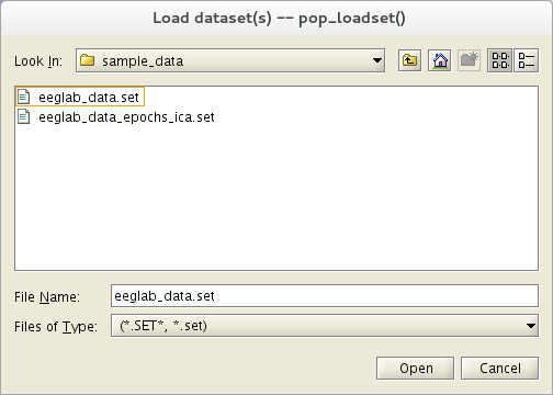
Select the tutorial file "eeglab_data.set up" distributed with the toolbox, and located in the "sample_data" folder of EEGLAB. And then press Open.

Expect upwardly channel locations

This section does not use the tutorial dataset. Its intent is to provide guidelines for automatically finding channel locations when channel names are known. For instance, when importing a Neuroscan, or a Biosemi channel locations file, channel names are often stored in the file header. EEGLAB will automatically read these channel labels. When you then call the channel editing window, the function volition wait upward x-x channel locations in a database of 385 defined channel labels, the file "Standard-ten-5-Cap385.sfp" in the "office/resource" sub-folder of the EEGLAB distribution. You may add additional standard channel locations to this file if you wish. As of 2021, the default channel location file for electrode position is the MNI file, which is best suited for source localization. Before 2021, it was the BESA spherical location file.

To load or edit channel location information independent in a dataset, select Edit → Channel locations. A dialog box (shown below) will appear, asking y'all if yous want to apply standard aqueduct locations based on the imported electrode position labels (for example, 'Fz') from a channel locations file using an extended International x-twenty Arrangement.

Image:Editchannelinfo_auto.png

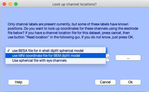
You may choose between several templates. If you lot intend to perform source localization, we strongly advise that yous select the second choice, "Utilize MNI coordinates for the BEM Dipfit model" (the commencement fix of 'BESA' coordinates was designed for a spherical BESA head model, now obsolete). Press Ok.

Command-line aqueduct location expect upwardly example

Below, we will build a channel structure using channel labels only, then volition call the channel editing window. In the MATLAB command window, type:

                          chanlocs              =              struct              (              'labels'              ,              {              'cz'              'c3'              'c4'              'pz'              'p3'              'p4'              'fz'              'f3'              'f4'              });              pop_chanedit              (              chanlocs              );

Then phone call Edit → Channel locations and look upwards channel locations. Printing Plot 2-D to plot the channel locations. Close the aqueduct editing window (using Cancel to discard the entered locations), then proceed to the next section.

Image:Topoplotlookup.gif

Load channel location from file

Reopen Edit → Aqueduct locations. In example it is not possible to look up channel locations based on their labels, or if you take a scanned electrode file available, press the Read Locations push button. For the current data file, you may select the sample channel locations file eeglab_chan32.locs (located in the sample_data sub-directory of the EEGLAB distribution).

Image:Loadchannellocation.png

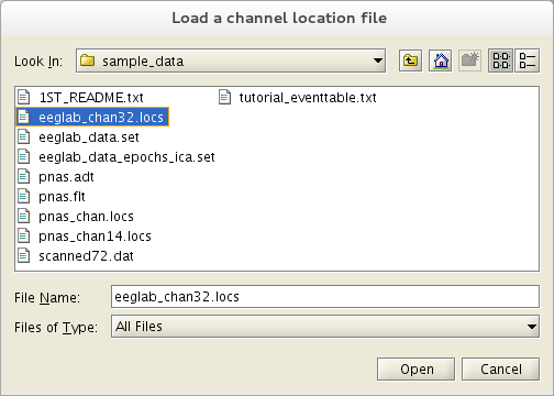
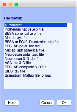
If you practise non specify the file format, the pop_chanedit.m function will try to employ the filename extension to assess its format. Press the button Read locs assist in the primary channel graphic interface window to view the supported formats. In the next pop-up window, simply press Ok.

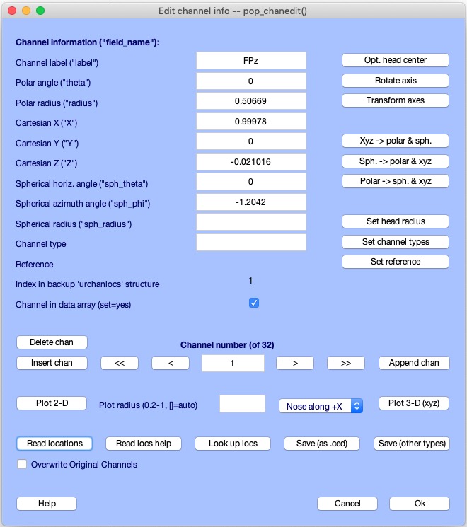
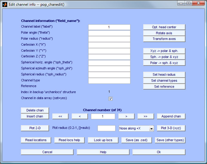
In the window below, you may ringlet through the aqueduct field values 1-by-1 using the < and → buttons, or in steps of 10 using << and >>.

The Set channel blazon push button allows you to enter a channel blazon associated with the aqueduct (for example, 'EEG', 'MEG', 'EMG', 'ECG', 'Events', etc.). Other EEGLAB functions may use channel types to restrict plotting and computation to a desired subset of channel types, allowing easier analysis of multi-modal datasets. Therefore, it is well worth the effort to add channel types to your information. It is essential to press Ok in the channel editing window above to actually import the channel locations. Note that in the main EEGLAB window, the aqueduct location flag now shows yes.

Viewing Channel Locations

Reopen Edit → Aqueduct locations if you closed it.

Plot channel location in 2-D

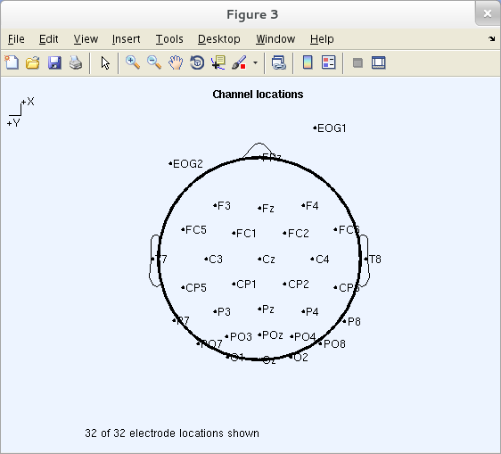
To visualize the 2-D locations of the channels, press Plot 2-D to a higher place the Read Locations button. Else, during an EEGLAB session, you may refer to a plot showing the aqueduct locations past selecting Plot → Aqueduct location → By proper noun. Either command pops up a window like that below. Nosotros recommend using the default settings.

Note: In this plot, click on whatsoever channel characterization to see its channel number.

Image:Channellocationname.png

Alert: Equating 'channel locations' with (single) electrode locations only makes sense when all channels use the same 'reference aqueduct.' An EEG channel signal is always the divergence between voltages at two (or more) electrodes – typically, electrodes "referred to" a reference channels. Equating the signal 'aqueduct location' to the location of one of the contributing electrodes is quite imprecise, every bit the aqueduct must be equally sensitive to potentials flowing to either of its two (or more) contributing scalp electrodes.

Electrodes plotted outside the head cartoon are electrodes located below the mid-head line (i.e., with a negative z (height) coordinate, 0 being the head's center). They are plotted outside the head drawing by convention. To plot scalp maps only within the head cartoon, enter 0.5 in the Plot radius edit box. In this example, the two centre electrodes will not be displayed nor taken into account when computing interpolated 2-D scalp maps for display or (in some cases) further processing. These settings are used for all scalp topographies plotted in EEGLAB.

If you do non see enough of the recorded field, set this dialogue box to i.0 to interpolate and show scalp maps including all possible scalp channel locations, with parts of the head below the (0.5) head equator shown in a 'skirt' or 'halo' region exterior the drawing head purlieus (more precise separate controls of which channel locations to plot are available from the control line: see the 'Assist' bulletin for the scalp map plotting function topoplot.1000).

Why are electrodes plotted outside of the head limits?

In the previous image, electrodes EOG1 and EOG2 are plotted beyond the head limit considering they extend below the caput center's horizontal plane. The topoplot.thou function plots them outside the cartoon caput that marks the (arc_length = 0.v) head-eye airplane. By default, all channels with location arc_lengths <= 1.0 (head bottom) are used for interpolation and are shown in the plot. From the command-line, topoplot.yard allows the user to specify the interpolation and plotting radii (intrad and plotrad) and the radius of the cartoon head (headrad). The headrad value should normally be kept at its physiologically right value (0.5), and for this reason, it is not possible to change it in the EEGLAB graphical interface.

When plotting in two-D, the distance of the electrode positions from the vertex is proportional to their (great circle) distance on the scalp to the vertex. This keeps the electrodes on the sides of the head from existence bunched together as they would exist in a peak-downward view of their positions. This great-circumvolve projection spreads out the positions of the lower electrodes. Thus, in the figure above, the (top) electrodes plotted on the lower portion of the 'skirt' are actually located on the lower part of the face. In the plot, they may appear spread out, whereas, in reality, they are bunched on the relatively narrow face surface. The combination of top-down and keen-circle projections allows the total component projection (or raw information scalp map) to exist seen clearly while allowing the viewer to estimate the bodily three-D locations of plot features. Importing continuous and epoched information

Plot aqueduct location in 3-D

To visualize the aqueduct locations in 3-D, press Plot 3-D (xyz). The window below will appear. The plotting box can exist rotated in 3-D using the mouse:

Image:3dlpotxyz.gif

Now the loaded channel labels and coordinates are displayed in the pop_chanedit.chiliad window. Annotation that the channel editor keeps polar to cartesian to spherical coordinate consistent. If you load a file containing polar coordinates for channel labels, they are automatically converted to cartesian and spherical coordinates. Y'all may change channel locations manually using the edit box provided for each aqueduct'south coordinates. Nevertheless, afterwards each modify, yous must update the other coordinate formats. For instance, if yous update the polar coordinates for ane channel, so press the polar → sph. & xyz button on the right of the pop_chanedit.m window (encounter above) to catechumen these values to other coordinate formats.

Supported Data Formats

Supported information formats are described in the assist bulletin of the readlocs.m role. Supported formats include:

'.loc', '.locs', '.eloc' file extensions: EEGLAB polar coordinate files
'.ced' extension: EEGLAB files containing polar, cartesian, and spherical coordinates
'.sph' extension: MATLAB spherical coordinates
'.elc' extension: Cartesian 3-D electrode coordinates scanned using the EETrak software.
'.elp' extension: Polhemus-.'elp' Cartesian coordinates
'.elp' extension: BESA-'.elp' spherical coordinates
'.xyz' extension: MATLAB/EEGLAB Cartesian coordinates
'.asc' and '.dat' extensions: Neuroscan-.'asc' or '.dat' Cartesian polar coordinates text file.
'.mat' extension: Brainstrom channel location file.
'.sfp' extension: BESA/EGI-xyz Cartesian coordinates

This readlocs.m office (which is called by the aqueduct editor) can also import custom channel location files where coordinate information is contained in dissimilar columns. Post-obit are examples of ASCII channel location data in EEGLAB-supported formats. Note that in all the examples below, the offset header line must not exist present.

Four channels from a polar coordinates file (with filename extension .loc, Practise not include the (calorie-free bluish) header line:

#	Deg.	Radius	Label
1	-xviii	,352	Fp1
ii	18	.352	Fp2
3	-90	,181	C3
four	90	,181	C4

The same locations, from a spherical coordinates file (estension, .sph ):

#	Azimut	Horiz.	Label
one	-63.36	-72	Fp1
two	63.36	72	Fp2
3	32.58	0	C3
4	32.58	0	C4

The same locations from a Cartesian coordinates file (extension, .xyz ):

#	X	Y	Z	Label
1	-0.8355	-0.2192	-0.5039	Fp1
ii	-0.8355	0.2192	0.5039	Fp2
iii	0.3956	0	-0.9184	C3
4	0.3956	0	0.9184	C4

Note using the Salvage (other type) button of the channel editing window also allows converting between channel location file formats.

For other template channel location files, see also the following web sites and FTP repositories (please edit this page to add more):

Sample files sent to u.s.
Neuroscan company spider web page
EGI channel location files
Easy-cap electrode locations
Piece of cake-cap electrode locations
BIOSEMI channel location files

Adjusting scanned iii-D channel locations

This section does not use the tutorial dataset. It intents to provide guidelines for importing channel locations measured in Cartesian coordinates using 3-D tracking devices (such every bit Polhemus). Utilise the EEGLAB menu Edit → Channel location or blazon the post-obit command on the MATLAB command line:

An empty channel editing window will appear:

Image:Editchannelinfo.jpg

Press the Read locations button and select the file scanned72.dat from the sample_data subfolder of the EEGLAB distribution. This is a aqueduct locations file measured with the Polhemus system using Neuroscan software (kindly supplied by Zoltan Mari). Utilize autodetect for the file format. When the file has been imported, set plotting radius to 0.6 to mask some reference points when plotting scalp topographies. So, press the Plot 2-D push. The following plot will pop up.

Image:Scanlocs1.gif

As y'all tin can meet, the measured 3-D channel coordinates may not be accurately distributed on the 2-D caput model. This is because the measured values have not been shifted to the head heart. To fix this problem, yous must first notice the head sphere center that best fits the imported 3-D electrode locations. To do and so, press the Opt. caput center (optimize caput center). The following window will popular up:

Image:Pop_chancenter.gif

Possibly, some of the channels should not be included in the head center optimization if they are not on the head and/or exercise non accept recorded locations. Enter electrodes indices to utilise (hither, 1:three 33 35 64:72) in the edit window. You may also press the Scan button above to select channels that are not on the head. When you press Ok in the browser window, the aqueduct indices will exist copied, as shown in the window in a higher place. Then press Ok. After the optimization has finished, press the Plot 2-D button once more.

Image:Scanlocs2.gif

In the view above, some aqueduct locations are all the same incorrect. For example, you may expect the aqueduct "Cz" to be at the vertex (i.east., the plot center). To adjust this, press the Rotate axis button. The following window will pop upward:

Image:Forcelocs.gif

Simply printing Ok to marshal channel 'Cz' to the vertex (past default). And so press the Plot ii-D push button in one case more to plot the scalp map again.

Image:Scanlocs3.gif

This department has illustrated operations you may want to perform to adapt measured 3-D channel locations for use in EEGLAB. You lot may now close the channel editing window.